Tutorial for BEMB with Simulated Data and the obs2prior Option

Author: Tianyu Du

Update: May. 6, 2022

This tutorial offers a simple simulation exercise to demonstrate how to use BEMB model and the power of BEMB's obs2prior feature. We highly recommend you to read the BEMB tutorial first.

The executable Jupyter notebook for this tutorial can be found here

import numpy as np
import pandas as pd
import torch
from torch_choice.data import ChoiceDataset
from bemb.model import LitBEMBFlex
from bemb.utils.run_helper import run
import matplotlib.pyplot as plt
import seaborn as sns

Simulate Dataset

We first specify the number of users and number of items in the dataset. The data_size denotes the number of user-item choice pairs to generate. Each user-item choice pair is called a purchasing record in our terminology, you can revise the data management tutorial.

Please note that the data_size is much smaller than num_users \(\times\) num_items and we are factorizing a spare matrix here.

num_users = 1500
num_items = 50
data_size = 1000

For each of data_size purchasing records, we randomly select one user as the decision maker. This information is stored the user_index tensor, which has length data_size.

user_index = torch.LongTensor(np.random.choice(num_users, size=data_size))

We further assign each individual some preferences so that our simulated is not totally random.

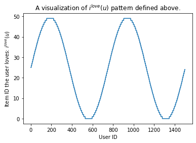
In particular, for each user \(u \in \{0, 1, \dots, num\_users - 1\}\), we assume \(u\) particularly loves the item \(i^*(u) \in \{0, 1, \dots, num\_item - 1\}\):

\[ i^{love}(u) = \left \lfloor \frac{\sin \left( \frac{u}{num\_users} \times 4 \times \pi \right) + 1}{2} \times num\_items \right \rfloor \]

The PREFERENCE dictionary maps each user \(u\) to the item she loves.

Us = np.arange(num_users)
Is = np.sin(np.arange(num_users) / num_users * 4 * np.pi)
Is = (Is + 1) / 2 * num_items
Is = Is.astype(int)

PREFERENCE = dict((u, i) for (u, i) in zip(Us, Is))

Even though the the formula looks complicated, the who-love-what pattern is quite simple. The figure below draws which item (y-axis) each user (x-axis) likes.

plt.close()
plt.plot(Us, Is)
plt.xlabel('User ID')
plt.ylabel('Item ID the user loves: $i^{love}(u)$')
plt.title('A visualization of $i^{love}(u)$ pattern defined above.')
plt.show()

To add some randomness, for each purchasing records, with 50\% chance, user \(u\) chooses the item \(i^*(u)\) she loves, and with 50\% of chance she chooses an item randomly.

# construct users.
item_index = torch.LongTensor(np.random.choice(num_items, size=data_size))

for idx in range(data_size):
    if np.random.rand() <= 0.5:
        item_index[idx] = PREFERENCE[int(user_index[idx])]

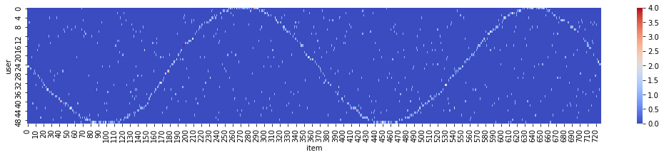
To have a visual inspection on the preference we added, we can plot a heat map indexed by (user, item) and visualize the frequency of bought items by each user. In the heat map below, each row represents the empirical distribution of items (x-axis) bought. Warmer color (red) indicates high purchasing frequencies, which shows the synthetic sin-curve of preference we enforced above.

df = pd.DataFrame(data={'item': item_index, 'user': user_index}).groupby(['item', 'user']).size().rename('size').reset_index()
df = df.pivot('item', 'user', 'size').fillna(0.0)

fig, ax = plt.subplots(figsize=(18, 3))
sns.heatmap(df.values, square=False, ax=ax, cmap='coolwarm')
ax.set(xlabel='item', ylabel='user')
fig.show()

Build the ChoiceDataset Object

We have created the user_index and item_index tensors, let's create a dataset object encompassing these tensors. Further, we split the dataset into train-validation-test subsets with ratio 80\%-10\%-10\%.

We wish to add some dummy user observables and item observables to that we can experiment the obs2prior feature of BEMB later.

The default item observable is simply the one-hot vector of the item identity.

The observable of a particular user is a one-hot vector with width num_items and one on the position of item this user loves (as mentioned previously).

user_obs = torch.zeros(num_users, num_items)
user_obs[torch.arange(num_users), Is] = 1

item_obs = torch.eye(num_items)

dataset = ChoiceDataset(user_index=user_index, item_index=item_index, user_obs=user_obs, item_obs=item_obs)

idx = np.random.permutation(len(dataset))
train_size = int(0.8 * len(dataset))
val_size = int(0.1 * len(dataset))
train_idx = idx[:train_size]
val_idx = idx[train_size: train_size + val_size]
test_idx = idx[train_size + val_size:]

dataset_list = [dataset[train_idx], dataset[val_idx], dataset[test_idx]]

No `session_index` is provided, assume each choice instance is in its own session.

dataset

ChoiceDataset(label=[], item_index=[1000], user_index=[1000], session_index=[1000], item_availability=[], user_obs=[1500, 50], item_obs=[50, 50], device=cpu)

Fitting the Model

We will be fitting a Bayesian matrix factorization model with utility form

$$ \mathcal{U}_{u, i} = \theta_u^\top \alpha_i $$ where \(\theta_u\) and \(\alpha_i\) are Bayesian variables. Please refer to the BEMB tutorial for a detailed description on how this kind of model works.

There are two options on the prior distributions of these Bayesian variables \(\theta_u\) and \(\alpha_i\). Firstly, we can simply use standard Gaussian as the prior distribution:

\[ \theta_u \overset{prior}{\sim} \mathcal{N}(\mathbf{0}, I) \quad \alpha_i \overset{prior}{\sim} \mathcal{N}(\mathbf{0}, I) \]

Alternatively, the prior can be chosen using a data-driven method called obs2prior. In particular, the mean of prior distribution can be a learnable linear function of user/item observables. Let \(X^{(user)}_u\) and \(X^{(item)}_i\) denote the observables of user \(u\) and item \(i\) respectively. The obs2prior-augmented prior distribution is the following:

\[ \theta_u \overset{prior}{\sim} \mathcal{N}(H X^{(user)}_u, I) \quad \alpha_i \overset{prior}{\sim} \mathcal{N}(W X^{(item)}_i, I) \]

where \(H\) and \(W\) are two learnable parameters.

def fit_model(obs2prior: bool):
    LATENT_DIM = 10  # the dimension of alpha and theta.
    bemb = LitBEMBFlex(
        learning_rate=0.03,  # set the learning rate, feel free to play with different levels.
        pred_item=True,  # let the model predict item_index, don't change this one.
        num_seeds=32,  # number of Monte Carlo samples for estimating the ELBO.
        utility_formula='theta_user * alpha_item',  # the utility formula.
        num_users=num_users,
        num_items=num_items,
        num_user_obs=dataset.user_obs.shape[1],
        num_item_obs=dataset.item_obs.shape[1],
        # whether to turn on obs2prior for each parameter.
        obs2prior_dict={'theta_user': obs2prior, 'alpha_item': obs2prior},
        # the dimension of latents, since the utility is an inner product of theta and alpha, they should have
        # the same dimension.
        coef_dim_dict={'theta_user': LATENT_DIM, 'alpha_item': LATENT_DIM}
    )

    # use GPU if available.
    if torch.cuda.is_available():
        bemb = bemb.to('cuda')

    # use the provided run helper to train the model.
    # we set batch size to be 5% of the data size, and train the model for 10 epochs.
    # there would be 20*10=200 gradient update steps in total.
    bemb = run(bemb, dataset_list, batch_size=len(dataset) // 20, num_epochs=50)

    # visualize the prediction.
    T = bemb.model.coef_dict['theta_user'].variational_mean_flexible.data
    A = bemb.model.coef_dict['alpha_item'].variational_mean_flexible.data
    fig, ax = plt.subplots(figsize=(18, 6))
    sns.heatmap((A @ T.T).numpy(), square=False, ax=ax, cmap='coolwarm')
    ax.set_title(f'obs2prior = {obs2prior}')
    fig.show()

fit_model(obs2prior=False)

BEMB: utility formula parsed:
[{'coefficient': ['theta_user', 'alpha_item'], 'observable': None}]


LOCAL_RANK: 0 - CUDA_VISIBLE_DEVICES: [0]

  | Name  | Type     | Params
-----------------------------------
0 | model | BEMBFlex | 31.0 K
-----------------------------------
31.0 K    Trainable params
0         Non-trainable params
31.0 K    Total params
0.124     Total estimated model params size (MB)


==================== model received ====================
Bayesian EMBedding Model with U[user, item, session] = theta_user * alpha_item
Total number of parameters: 31000.
With the following coefficients:
ModuleDict(
  (theta_user): BayesianCoefficient(num_classes=1500, dimension=10, prior=N(0, I))
  (alpha_item): BayesianCoefficient(num_classes=50, dimension=10, prior=N(0, I))
)
[]
==================== data set received ====================
[Training dataset] ChoiceDataset(label=[], item_index=[800], user_index=[800], session_index=[800], item_availability=[], user_obs=[1500, 50], item_obs=[50, 50], device=cpu)
[Validation dataset] ChoiceDataset(label=[], item_index=[100], user_index=[100], session_index=[100], item_availability=[], user_obs=[1500, 50], item_obs=[50, 50], device=cpu)
[Testing dataset] ChoiceDataset(label=[], item_index=[100], user_index=[100], session_index=[100], item_availability=[], user_obs=[1500, 50], item_obs=[50, 50], device=cpu)
==================== train the model ====================
time taken: 40.19812321662903
==================== test performance ====================



Testing: 0it [00:00, ?it/s]


─────────────────────────────────────────────────────────────────────────────────────────────────────────────────────────────────────────────────────────────────────────────────────────────────────────────────────────────────────────────
       Test metric             DataLoader 0
─────────────────────────────────────────────────────────────────────────────────────────────────────────────────────────────────────────────────────────────────────────────────────────────────────────────────────────────────────────────
        test_acc                   0.02
         test_ll            -3.912011494636536
─────────────────────────────────────────────────────────────────────────────────────────────────────────────────────────────────────────────────────────────────────────────────────────────────────────────────────────────────────────────

fit_model(obs2prior=True)

GPU available: True, used: True
TPU available: False, using: 0 TPU cores
IPU available: False, using: 0 IPUs
HPU available: False, using: 0 HPUs
LOCAL_RANK: 0 - CUDA_VISIBLE_DEVICES: [0]

  | Name  | Type     | Params
-----------------------------------
0 | model | BEMBFlex | 33.0 K
-----------------------------------
33.0 K    Trainable params
0         Non-trainable params
33.0 K    Total params
0.132     Total estimated model params size (MB)


BEMB: utility formula parsed:
[{'coefficient': ['theta_user', 'alpha_item'], 'observable': None}]
==================== model received ====================
Bayesian EMBedding Model with U[user, item, session] = theta_user * alpha_item
Total number of parameters: 33000.
With the following coefficients:
ModuleDict(
  (theta_user): BayesianCoefficient(num_classes=1500, dimension=10, prior=N(H*X_obs(H shape=torch.Size([10, 50]), X_obs shape=50), Ix1.0))
  (alpha_item): BayesianCoefficient(num_classes=50, dimension=10, prior=N(H*X_obs(H shape=torch.Size([10, 50]), X_obs shape=50), Ix1.0))
)
[]
==================== data set received ====================
[Training dataset] ChoiceDataset(label=[], item_index=[800], user_index=[800], session_index=[800], item_availability=[], user_obs=[1500, 50], item_obs=[50, 50], device=cpu)
[Validation dataset] ChoiceDataset(label=[], item_index=[100], user_index=[100], session_index=[100], item_availability=[], user_obs=[1500, 50], item_obs=[50, 50], device=cpu)
[Testing dataset] ChoiceDataset(label=[], item_index=[100], user_index=[100], session_index=[100], item_availability=[], user_obs=[1500, 50], item_obs=[50, 50], device=cpu)
==================== train the model ====================
time taken: 40.98820662498474
==================== test performance ====================



Testing: 0it [00:00, ?it/s]


─────────────────────────────────────────────────────────────────────────────────────────────────────────────────────────────────────────────────────────────────────────────────────────────────────────────────────────────────────────────
       Test metric             DataLoader 0
─────────────────────────────────────────────────────────────────────────────────────────────────────────────────────────────────────────────────────────────────────────────────────────────────────────────────────────────────────────────
        test_acc                   0.47
         test_ll            -3.126977977901697
─────────────────────────────────────────────────────────────────────────────────────────────────────────────────────────────────────────────────────────────────────────────────────────────────────────────────────────────────────────────

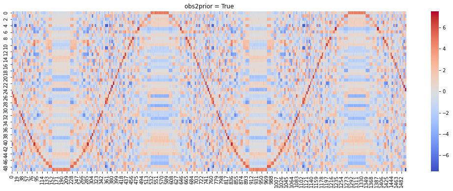
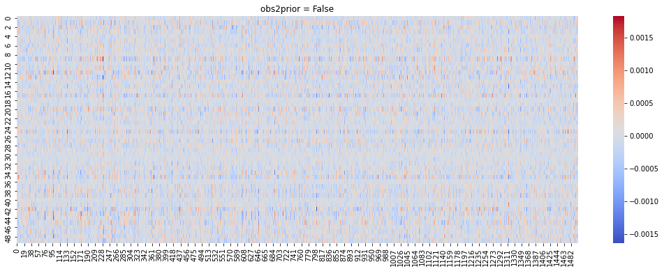
Now we compare the difference between two options of prior distributions. We provide a fit_model helper function to train and visualize the model. You can go through fit_model method to have a preliminary understanding on how to train a BEMB model.

Visualization: The method visualize the fitted model by plotting \(\theta_u^\top \alpha_i\) for all pairs of user \(u\) and item \(i\) on a heat map. The sine-curve on the heat map indicates the model successfully recovered the preference pattern we added.